GrrrrrlScientist struck me with first ever blog meme (woo-hoo!). I had to participate, but it took me a bit of time thanks to hardware problems and an influx of spawning cod. So. Here we go...
The Rules are as follows:
Seven Random or Weird Things About Me:
Seven Random Bloggers whom I read;
Read more!
Wednesday, 12 December 2007
Oooh! Struck by a blog meme!

Monday, 10 December 2007
BBC report filtered out
Hmmm. If you're reading this, your globus pallidus is being underused.
Actually, it's somehow comforting that there is a part of the brain dedicated to ignoring things. And another dedicated to deciding what's irrelevant. But somehow Henry always seems to slip past that one.
Read more!
Wednesday, 5 December 2007
Focus on DIC
This is something that's only of interest to Bayesians, so the rest of you can look away.
In a couple of analyses with BUGS, I've seen comparisons of DIC from different models, and the values have been almost exactly the same. This sort of thing is suspicious, and eventually I worked out why. I thought it was worth posting about this, so that everyone else can share The Secret.
It's best to explain the problem with an example (the complete R code for this is below). I simulated a couple of simple hierarchical models, so
Yij ~ N(θi, σy2)
θi ~ N(μi, σθ2)
(j =1,...,n, i=1,...,m. There are m groups, each with n observations). I then had two models for μi:
Model 1
μi = φ + β (i-5.5)
Model 2
μi = φ
The first model has a covariate (cunningly equal to the identity of the group), and the second has none. The data are plotted below. The effect of the covariate is clear, so DIC should be able to pick it up.
Now, I fit each of the models to each data set. This is easy running it through the R2WinBUGS package in R. From this I can extract the DIC:
Data 1
Model 1 DIC: 1464.0 pD: 10.9
Model 2 DIC: 1464.4 pD: 11.2
Data 2
Model 1 DIC: 1407.7 pD: 10.9
Model 2 DIC: 1407.7 pD: 10.9
So, in both cases the DIC is the same (for Data 2 the difference is in the third decimal place!). But for Data 1, Model 1 should be better - hey, we can see it on the figure! So, what's going on?
We can get a clue from plotting the posteriors for μi from the groups, from the two models:
Only the error bars are plotted (i.e. plus/minus 1 posterior standard deviation), and the 1:1 line is drawn in a fetching shade called "hotpink". Obviously the models are predicting the same means for the groups, and hence we will get the same deviance. We can see why this is happening from the group-level standard deviations (σθ2, posterior means and standard errors in parentheses):
Data 1
Model 1: 0.87 (0.280)
Model 2: 4.4 (1.31)
Data 2
Model 1: 1.1 (0.34)
Model 2: 1.1 (0.31)
So, for the data where there is a trend, but none is fitted, σθ2 is much larger - essentially, the lack of the linear trend is compensated by the increase in variance. The difference is not in the model for θ at all, but higher in the hierarchy (or hier in the higherarchy?).
Of course, this is obvious from looking at the models. The solution is to change the focus, from θ to φ and &beta. This then means calculating the marginal deviance, marginalising over θ, i.e. looking at P(Y | φ, β) and integrating over P(θ | Y). This can be done analytically (Hat-tip to David Spiegelhalter for correcting my errors, and refraining from making any justified comments about my mathematical ability!), whence we find that the deviance can be calculated because
barYi. ~ N(μi, σy2/n + σθ2) )
when we do this, we get these results:
Data 1
Model 1 DIC: 26.9 pD: 2.7
Model 2 DIC: 57.8 pD: 1.7
Data 2
Model 1 DIC: 30.9 pD: 2.6
Model 2 DIC: 30.3 pD: 1.7
Now this makes more sense, for the data with an effect, the DIC massively favours the correct model. Without the effect in the data, the DIC is pretty similar. In both cases, also note that pD is larger by 1 for the model with 1 extra parameter. Which is what should happen!
What lessons can we draw from this? Firstly, that DIC is not an automatic panacea - you do have to focus it on the right part of the model. If the focus is not at the level immediately above the data (i.e. θ here), then you can't use the DIC given by BUGS. The correctly focussed DIC is more complex to get at: you have to calculate it yourself. For more complex models this might be awkward, if there are no analytical results, then the parameters to be integrated out have to be simulated, for example by MCMC. But this requires some further thought...
library(R2WinBUGS)
# Simulate data
Cov=1:10
Group = rep(Cov, each=50)
beta = 1
# With covariate
GrpMean1=rnorm(length(Cov), beta*Cov, 1)
Value1=rnorm(length(Group), GrpMean1[Group], 1)
DataToBUGS1=list(N=length(Value1), NGrp=length(Cov), Group=Group, Y=Value1)
# Without covariate
GrpMean2=rnorm(length(Cov), 5.5, 1)
Value2=rnorm(length(Group), GrpMean2[Group], 1)
DataToBUGS2=list(N=length(Value2), NGrp=length(Cov), Group=Group, Y=Value2)
# Plot the data
# png("C:/Bob/Blog/Data.png", width = 960, height = 480)
par(mfrow=c(1,2), mar=c(2.1,2.1,1.1,1.1), oma=c(2,2,0,0), las=1)
plot(jitter(Group), Value1, pch=3, col="grey70")
points(Cov, GrpMean1, col=1, pch=3, cex=1.5)
plot(jitter(Group), Value2, pch=3, col="grey70")
points(Cov, GrpMean2, col=1, pch=3, cex=1.5)
mtext("Group", 1, outer=T)
mtext("Y", 2, outer=T)
#dev.off()
# Write BUGS models to files
model1 <- function(){
for (i in 1:N){ Y[i] ~ dnorm(muGrp[Group[i]], tau.y) }
for (j in 1:NGrp){
muGrp[j] ~ dnorm(muG[j], tau.Grp)
muG[j] <- mu0 + betaGrp*(j-5.5)
}
mu0 ~ dnorm (0.0, 1.0E-6)
betaGrp ~ dnorm (0.0, 1.0E-6)
tau.y <- pow(sigma.y, -2)
sigma.y ~ dunif (0, 1000)
tau.Grp <- pow(sigma.Grp, -2)
sigma.Grp ~ dunif (0, 1000)
}
write.model(model1, "C:/Bob/Blog/model1.txt")
model2 <- function(){
for (i in 1:N){ Y[i] ~ dnorm(muGrp[Group[i]], tau.y) }
for (j in 1:NGrp){ muGrp[j] ~ dnorm(mu0, tau.Grp) }
mu0 ~ dnorm (0.0, 1.0E-6)
tau.y <- pow(sigma.y, -2)
sigma.y ~ dunif (0, 1000)
tau.Grp <- pow(sigma.Grp, -2)
sigma.Grp ~ dunif (0, 1000)
}
write.model(model2, "C:/Bob/Blog/model2.txt")
# Initial values
Inits1=list(list(mu0=0, betaGrp=1, sigma.Grp=5, sigma.y=1), list(mu0=2, betaGrp=0, sigma.Grp=5, sigma.y=1) )
Inits2=list(list(mu0=0, sigma.Grp=5, sigma.y=1), list(mu0=2, sigma.Grp=5, sigma.y=1) )
# Fit the models
# Data 1, Model 1
Data1Model1.post=openbugs(DataToBUGS1, inits=Inits1, c("mu0", "muGrp", "betaGrp", "sigma.y", "sigma.Grp"), model.file = "C:/Bob/Blog/model1.txt", n.chains = 2, n.iter = 11000, n.burnin = 1000, n.thin = 10)
# Data 1, Model 2 (no slope in model)
Data1Model2.post=openbugs(DataToBUGS1, inits=Inits2, c("mu0", "muGrp", "sigma.y", "sigma.Grp"), model.file = "C:/Bob/Blog/model2.txt", n.chains = 2, n.iter = 11000, n.burnin = 1000, n.thin = 10)
# Data 2, Model 1
Data2Model1.post=openbugs(DataToBUGS2, inits=Inits1, c("mu0", "muGrp", "betaGrp", "sigma.y", "sigma.Grp"), model.file = "C:/Bob/Blog/model1.txt", n.chains = 2, n.iter = 11000, n.burnin = 1000, n.thin = 10)
# Data 2, Model 2 (no slope in model)
Data2Model2.post=openbugs(DataToBUGS2, inits=Inits2, c("mu0", "muGrp", "betaGrp", "sigma.y", "sigma.Grp"), model.file = "C:/Bob/Blog/model2.txt", n.chains = 2, n.iter = 11000, n.burnin = 1000, n.thin = 10)
print(Data1Model1.post)
print(Data1Model2.post)
print(Data2Model1.post)
print(Data2Model2.post)
# Plot mu
# png("C:/Bob/Blog/Theta.png", width = 960, height = 480)
par(mfrow=c(1,2), mar=c(2.1,2.1,1.1,1.1), oma=c(2,2,1,0), las=1)
plot(Data1Model1.post$mean$muGrp, Data1Model2.post$mean$muGrp, type="n", main="Data 1")
segments(Data1Model1.post$mean$muGrp,Data1Model2.post$mean$muGrp-Data1Model2.post$sd$muGrp, Data1Model1.post$mean$muGrp, Data1Model2.post$mean$muGrp+Data1Model2.post$sd$muGrp)
segments(Data1Model1.post$mean$muGrp-Data1Model1.post$sd$muGrp, Data1Model2.post$mean$muGrp, Data1Model1.post$mean$muGrp+Data1Model1.post$sd$muGrp, Data1Model2.post$mean$muGrp)
abline(0,1, col="hotpink")
plot(Data2Model1.post$mean$muGrp, Data2Model2.post$mean$muGrp, type="n", main="Data 2")
segments(Data2Model1.post$mean$muGrp, Data2Model2.post$mean$muGrp-Data2Model2.post$sd$muGrp, Data2Model1.post$mean$muGrp, Data2Model2.post$mean$muGrp+Data2Model2.post$sd$muGrp)
segments(Data2Model1.post$mean$muGrp-Data2Model1.post$sd$muGrp, Data2Model2.post$mean$muGrp, Data2Model1.post$mean$muGrp+Data2Model1.post$sd$muGrp, Data2Model2.post$mean$muGrp)
abline(0,1, col="hotpink")
mtext(expression(paste(theta[i], ", Model 1", sep="")), 1, outer=T)
mtext(expression(paste(theta[i], ", Model 2", sep="")), 2, outer=T, las=0)
#dev.off()
####################################################################### DevCalc1=function(mcmc, data) {
NamesGrp=paste("muGrp[", data$Group, "]", sep="")
-2*sum(dnorm(data$Y, mcmc[NamesGrp], mcmc["sigma.y"], log=TRUE))
}
DevCalc2=function(mcmc, data) {
Mean=unlist(tapply(data$Y, list(data$Group), mean))
Mu=mcmc["mu0"]
N=length(data$Group)/length(unique(data$Group))
-2*sum(dnorm(Mean, Mu, sqrt((mcmc["sigma.y"]^2)/N + mcmc["sigma.Grp"]^2), log=TRUE)) }
DevCalc2beta=function(mcmc, data) {
Mean=unlist(tapply(data$Y, list(data$Group), mean))
Mu=mcmc["mu0"] + mcmc["betaGrp"]*(as.numeric(names(Mean)) - 5.5)
N=length(data$Group)/length(unique(data$Group))
-2*sum(dnorm(Mean, Mu, sqrt((mcmc["sigma.y"]^2)/N + mcmc["sigma.Grp"]^2), log=TRUE))
}
DIC.calc=function(dat, mcmc, func) {
Dev=apply(mcmc$sims.array, c(1,2), func, data=dat)
mean=apply(mcmc$sims.array, 3, mean)
pD=mean(Dev) - func(mean, dat)
DIC=mean(Dev) + pD
return(list(DIC=DIC, pD=pD, Dbar=mean(Dev)))
}
PrintDIC=function(DIC, Label) { cat(Label, " DIC:", DIC$DIC, " pD:", DIC$pD, "\n")}
# Focus on theta
DIC.D1M1=DIC.calc(DataToBUGS1, Data1Model1.post, DevCalc1) DIC.D1M2=DIC.calc(DataToBUGS1, Data1Model2.post, DevCalc1)
DIC.D2M1=DIC.calc(DataToBUGS2, Data2Model1.post, DevCalc1)
DIC.D2M2=DIC.calc(DataToBUGS2, Data2Model2.post, DevCalc1)
PrintDIC(DIC.D1M1, "Data 1, Model 1")
PrintDIC(DIC.D1M2, "Data 1, Model 2")
PrintDIC(DIC.D2M1, "Data 2, Model 1")
PrintDIC(DIC.D2M2, "Data 2, Model 2")
# Focus on phi
DIC2.D1M1=DIC.calc(DataToBUGS1, Data1Model1.post, DevCalc2beta)
DIC2.D1M2=DIC.calc(DataToBUGS1, Data1Model2.post, DevCalc2)
DIC2.D2M1=DIC.calc(DataToBUGS2, Data2Model1.post, DevCalc2beta)
DIC2.D2M2=DIC.calc(DataToBUGS2, Data2Model2.post, DevCalc2)
PrintDIC(DIC2.D1M1, "Data 1, Model 1")
PrintDIC(DIC2.D1M2, "Data 1, Model 2")
PrintDIC(DIC2.D2M1, "Data 2, Model 1")
PrintDIC(DIC2.D2M2, "Data 2, Model 2")
Read more!
Tuesday, 4 December 2007
Finnish curiosities
The Finns are a curious people. This morning I got a phone call asking me if I owned a TV.
I don't. End of conversation. We actually spent longer ascertaining that the conversation had to be in Enlgish.
Read more!
Saturday, 24 November 2007
The Beast is Happy
The beast is evil. How can you not like him when he's this happy?
But why is he so happy...
Because he has a new prime minister. I told him the guy's name is Rudd, and he thought it was great having a fish as PM - if he's a failure, some lucky moggie can eat him.
I guess this explains why he was never impressed with Bush in the US - he has a self-cleaning litter tray already.
Read more!
Monday, 12 November 2007
Damn, it was only spam
Drum Snail Bible Necklace Festival
Snail Foot Dung Rope Leather jacket
Is the leather jacket made from a drum snail, one wonders.
Powered by ScribeFire.
Sunday, 4 November 2007
Thrilling
Some people have far too much time on their hands. They could be doing something profitable, like writing a blog. Instead...
They re-make Jacko's Thriller in lego.
Incidentally, I came across this whilst trying to find a photo to illustrate oozing.
Read more!